Variance Reduction - Weight Windows#
Creating and utilizing a weight window to accelerate deep shielding simulations#
This example simulates a shield room / bunker with corridor entrance and a neutron source in the center of the room. This example implements a single step of the Magic method of weight window generation.
In this tutorial we shall focus on generating a weight window to accelerate the simulation of particles through a shield.
Weight Windows are found using the MAGIC method and used to accelerate the simulation.
The variance reduction method used for this simulation is well documented in the OpenMC documentation https://docs.openmc.org/en/stable/methods/neutron_physics.html
The MAGIC method is well described in the original publication https://scientific-publications.ukaea.uk/wp-content/uploads/Published/INTERN1.pdf
First we import openmc and other packages needed for the example and configure the nuclear data path
import time  # used to time the simulation
import numpy as np

from matplotlib import pyplot as plt
from matplotlib.colors import LogNorm  # used for plotting log scale graphs

import openmc
from pathlib import Path
# Setting the cross section path to the correct location in the docker image.
# If you are running this outside the docker image you will have to change this path to your local cross section path.
openmc.config['cross_sections'] = Path.home() / 'nuclear_data' / 'cross_sections.xml'
We create a couple of materials for the simulation
mat_air = openmc.Material(name="Air")
mat_air.add_element("N", 0.784431)
mat_air.add_element("O", 0.210748)
mat_air.add_element("Ar", 0.0046)
mat_air.set_density("g/cc", 0.001205)

mat_concrete = openmc.Material()
mat_concrete.add_element("H",0.168759)
mat_concrete.add_element("C",0.001416)
mat_concrete.add_element("O",0.562524)
mat_concrete.add_element("Na",0.011838)
mat_concrete.add_element("Mg",0.0014)
mat_concrete.add_element("Al",0.021354)
mat_concrete.add_element("Si",0.204115)
mat_concrete.add_element("K",0.005656)
mat_concrete.add_element("Ca",0.018674)
mat_concrete.add_element("Fe",0.00426)
mat_concrete.set_density("g/cm3", 2.3)

materials = openmc.Materials([mat_air, mat_concrete])
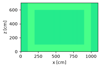
Now we define and plot the geometry. This geometry is defined by parameters for every width and height. The parameters input into the geometry in a stacked manner so they can easily be adjusted to change the geometry without creating overlapping cells.
width_a = 100
width_b = 100
width_c = 500
width_d = 100
width_e = 100
width_f = 100
width_g = 100

depth_a = 100
depth_b = 100
depth_c = 700
depth_d = 600
depth_e = 100
depth_f = 100

height_j = 100
height_k = 500
height_l = 100

xplane_0 = openmc.XPlane(x0=0, boundary_type="vacuum")
xplane_1 = openmc.XPlane(x0=xplane_0.x0 + width_a)
xplane_2 = openmc.XPlane(x0=xplane_1.x0 + width_b)
xplane_3 = openmc.XPlane(x0=xplane_2.x0 + width_c)
xplane_4 = openmc.XPlane(x0=xplane_3.x0 + width_d)
xplane_5 = openmc.XPlane(x0=xplane_4.x0 + width_e)
xplane_6 = openmc.XPlane(x0=xplane_5.x0 + width_f)
xplane_7 = openmc.XPlane(x0=xplane_6.x0 + width_g, boundary_type="vacuum")

yplane_0 = openmc.YPlane(y0=0, boundary_type="vacuum")
yplane_1 = openmc.YPlane(y0=yplane_0.y0 + depth_a)
yplane_2 = openmc.YPlane(y0=yplane_1.y0 + depth_b)
yplane_3 = openmc.YPlane(y0=yplane_2.y0 + depth_c)
yplane_4 = openmc.YPlane(y0=yplane_3.y0 + depth_d)
yplane_5 = openmc.YPlane(y0=yplane_4.y0 + depth_e)
yplane_6 = openmc.YPlane(y0=yplane_5.y0 + depth_f, boundary_type="vacuum")

zplane_1 = openmc.ZPlane(z0=0, boundary_type="vacuum")
zplane_2 = openmc.ZPlane(z0=zplane_1.z0 + height_j)
zplane_3 = openmc.ZPlane(z0=zplane_2.z0 + height_k)
zplane_4 = openmc.ZPlane(z0=zplane_3.z0 + height_l, boundary_type="vacuum")

outside_left_region = +xplane_0 & -xplane_1 & +yplane_1 & -yplane_5 & +zplane_1 & -zplane_4
wall_left_region = +xplane_1 & -xplane_2 & +yplane_2 & -yplane_4 & +zplane_2 & -zplane_3
wall_right_region = +xplane_5 & -xplane_6 & +yplane_2 & -yplane_5 & +zplane_2 & -zplane_3
wall_top_region = +xplane_1 & -xplane_4 & +yplane_4 & -yplane_5 & +zplane_2 & -zplane_3
outside_top_region = +xplane_0 & -xplane_7 & +yplane_5 & -yplane_6 & +zplane_1 & -zplane_4
wall_bottom_region = +xplane_1 & -xplane_6 & +yplane_1 & -yplane_2 & +zplane_2 & -zplane_3
outside_bottom_region = +xplane_0 & -xplane_7 & +yplane_0 & -yplane_1 & +zplane_1 & -zplane_4
wall_middle_region = +xplane_3 & -xplane_4 & +yplane_3 & -yplane_4 & +zplane_2 & -zplane_3
outside_right_region = +xplane_6 & -xplane_7 & +yplane_1 & -yplane_5 & +zplane_1 & -zplane_4

room_region = +xplane_2 & -xplane_3 & +yplane_2 & -yplane_4 & +zplane_2 & -zplane_3
gap_region = +xplane_3 & -xplane_4 & +yplane_2 & -yplane_3 & +zplane_2 & -zplane_3
corridor_region = +xplane_4 & -xplane_5 & +yplane_2 & -yplane_5 & +zplane_2 & -zplane_3

roof_region = +xplane_1 & -xplane_6 & +yplane_1 & -yplane_5 & +zplane_1 & -zplane_2
floor_region = +xplane_1 & -xplane_6 & +yplane_1 & -yplane_5 & +zplane_3 & -zplane_4

outside_left_cell = openmc.Cell(region=outside_left_region, fill=mat_air)
outside_right_cell = openmc.Cell(region=outside_right_region, fill=mat_air)
outside_top_cell = openmc.Cell(region=outside_top_region, fill=mat_air)
outside_bottom_cell = openmc.Cell(region=outside_bottom_region, fill=mat_air)
wall_left_cell = openmc.Cell(region=wall_left_region, fill=mat_concrete)
wall_right_cell = openmc.Cell(region=wall_right_region, fill=mat_concrete)
wall_top_cell = openmc.Cell(region=wall_top_region, fill=mat_concrete)
wall_bottom_cell = openmc.Cell(region=wall_bottom_region, fill=mat_concrete)
wall_middle_cell = openmc.Cell(region=wall_middle_region, fill=mat_concrete)
room_cell = openmc.Cell(region=room_region, fill=mat_air)
gap_cell = openmc.Cell(region=gap_region, fill=mat_air)
corridor_cell = openmc.Cell(region=corridor_region, fill=mat_air)

roof_cell = openmc.Cell(region=roof_region, fill=mat_concrete)
floor_cell = openmc.Cell(region=floor_region, fill=mat_concrete)

geometry = openmc.Geometry(
    [
        outside_bottom_cell,
        outside_top_cell,
        outside_left_cell,
        outside_right_cell,
        wall_left_cell,
        wall_right_cell,
        wall_top_cell,
        wall_bottom_cell,
        wall_middle_cell,
        room_cell,
        gap_cell,
        corridor_cell,
        roof_cell,
        floor_cell,
    ]
)
Now we plot the geometry and color by materials.
plot = geometry.plot(basis='xz',  color_by='material')
plot.figure.savefig('geometry_top_down_view.png', bbox_inches="tight")
Next we create a point source, this also uses the same geometry parameters to place in the center of the room regardless of the values of the parameters.
# location of the point source
source_x = width_a + width_b + width_c * 0.5
source_y = depth_a + depth_b + depth_c * 0.75
source_z = height_j + height_k * 0.5
space = openmc.stats.Point((source_x, source_y, source_z))

angle = openmc.stats.Isotropic()

# all (100%) of source particles are 2.5MeV energy
energy = openmc.stats.Discrete([2.5e6], [1.0])

source = openmc.IndependentSource(space=space, angle=angle, energy=energy)
source.particle = "neutron"
Next we create a mesh that encompasses the entire geometry and scores neutron flux
mesh = openmc.RegularMesh().from_domain(geometry)
mesh.dimension = (500, 500, 1)

mesh_filter = openmc.MeshFilter(mesh, filter_id=1)
particle_filter = openmc.ParticleFilter('neutron', filter_id=2)

flux_tally = openmc.Tally(name="flux tally")
flux_tally.filters = [mesh_filter, particle_filter]
flux_tally.scores = ["flux"]
flux_tally.id = 42  # we set the ID because we need to access this later

tallies = openmc.Tallies([flux_tally])
Creates the simulation settings
settings = openmc.Settings()

settings.run_mode = "fixed source"
settings.source = source
settings.particles = 80000
settings.batches = 5
# no need to write the tallies.out file which saves space and time when large meshes are used
settings.output = {'tallies': False}
Creates and exports the model
model = openmc.Model(geometry, materials, settings, tallies)
We are going to plot the mesh results with and without weight windows so lets write a function for the plotting
def run_and_plot(model: openmc.Model, image_filename: str) -> openmc.StatePoint:

    for f in Path('.').glob('*.h5'):
        f.unlink(missing_ok=True)
    sp_filename = model.run()

    with openmc.StatePoint(sp_filename) as sp:
        flux_tally = sp.get_tally(name="flux tally")

    mesh_extent = mesh.bounding_box.extent['xy']

    # create a plot of the mean flux values
    flux_mean = flux_tally.get_reshaped_data(value='mean', expand_dims=True).squeeze()

    fig, (ax1, ax2) = plt.subplots(ncols=2, figsize=(10, 5))
    ax1.imshow(
        flux_mean.T,
        origin="lower",
        extent=mesh_extent,
        norm=LogNorm(),
    )

    ax1 = model.plot(
        outline='only',
        extent=model.bounding_box.extent['xz'],
        axes=ax1,  # Use the same axis as ax1\n",
        pixels=10_000_000,  #avoids rounded corners on outline
        color_by='material',
    )
    ax1.set_title("Flux Mean")

    # create a plot of the flux relative error
    flux_std_dev = flux_tally.get_reshaped_data(value='std_dev', expand_dims=True).squeeze()
    ax2.imshow(
        flux_std_dev.T,
        origin="lower",
        extent=mesh_extent,
        norm=LogNorm(),
    )

    ax2 = model.plot(
        outline='only',
        extent=model.bounding_box.extent['xz'],
        axes=ax2,  # Use the same axis as ax2\n",
        pixels=10_000_000,  #avoids rounded corners on outline
        color_by='material',
    )
    ax2.set_title("Flux Std. Dev.")

    plt.savefig(image_filename)
    return sp
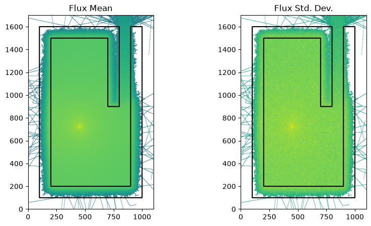
Now we run the model without weight windows
# this helps time the simulation
t0 = time.time()

# delete the old summary file if it exists
Path('summary.h5').unlink(missing_ok=True)

run_and_plot(model, 'no_ww_statepoint_filename.png')

print(f'total time without weight windows {int(time.time()-t0)}s')
                                %%%%%%%%%%%%%%%
                           %%%%%%%%%%%%%%%%%%%%%%%%
                        %%%%%%%%%%%%%%%%%%%%%%%%%%%%%%
                      %%%%%%%%%%%%%%%%%%%%%%%%%%%%%%%%%%
                    %%%%%%%%%%%%%%%%%%%%%%%%%%%%%%%%%%%%%%
                   %%%%%%%%%%%%%%%%%%%%%%%%%%%%%%%%%%%%%%%%
                                    %%%%%%%%%%%%%%%%%%%%%%%%
                                     %%%%%%%%%%%%%%%%%%%%%%%%
                 ###############      %%%%%%%%%%%%%%%%%%%%%%%%
                ##################     %%%%%%%%%%%%%%%%%%%%%%%
                ###################     %%%%%%%%%%%%%%%%%%%%%%%
                ####################     %%%%%%%%%%%%%%%%%%%%%%
                #####################     %%%%%%%%%%%%%%%%%%%%%
                ######################     %%%%%%%%%%%%%%%%%%%%
                #######################     %%%%%%%%%%%%%%%%%%
                 #######################     %%%%%%%%%%%%%%%%%
                 ######################     %%%%%%%%%%%%%%%%%
                  ####################     %%%%%%%%%%%%%%%%%
                    #################     %%%%%%%%%%%%%%%%%
                     ###############     %%%%%%%%%%%%%%%%
                       ############     %%%%%%%%%%%%%%%
                          ########     %%%%%%%%%%%%%%
                                      %%%%%%%%%%%

                 | The OpenMC Monte Carlo Code
       Copyright | 2011-2026 MIT, UChicago Argonne LLC, and contributors
         License | https://docs.openmc.org/en/latest/license.html
         Version | 0.15.3-dev485
     Commit Hash | 6704e4786a743611baac5d693943f67f7479ee47
       Date/Time | 2026-06-17 21:41:28
  OpenMP Threads | 4

 Reading model XML file 'model.xml' ...
 Reading cross sections XML file...
 Reading N14 from /home/runner/nuclear_data/neutron/N14.h5
 Reading N15 from /home/runner/nuclear_data/neutron/N15.h5
 Reading O16 from /home/runner/nuclear_data/neutron/O16.h5
 Reading O17 from /home/runner/nuclear_data/neutron/O17.h5
 Reading O18 from /home/runner/nuclear_data/neutron/O18.h5
 Reading Ar36 from /home/runner/nuclear_data/neutron/Ar36.h5
 WARNING: Negative value(s) found on probability table for nuclide Ar36 at 294K
 Reading Ar38 from /home/runner/nuclear_data/neutron/Ar38.h5
 Reading Ar40 from /home/runner/nuclear_data/neutron/Ar40.h5
 Reading H1 from /home/runner/nuclear_data/neutron/H1.h5
 Reading H2 from /home/runner/nuclear_data/neutron/H2.h5
 Reading C12 from /home/runner/nuclear_data/neutron/C12.h5
 Reading C13 from /home/runner/nuclear_data/neutron/C13.h5
 Reading Na23 from /home/runner/nuclear_data/neutron/Na23.h5
 Reading Mg24 from /home/runner/nuclear_data/neutron/Mg24.h5
 Reading Mg25 from /home/runner/nuclear_data/neutron/Mg25.h5
 Reading Mg26 from /home/runner/nuclear_data/neutron/Mg26.h5
Reading Al27 from /home/runner/nuclear_data/neutron/Al27.h5
Reading Si28 from /home/runner/nuclear_data/neutron/Si28.h5
Reading Si29 from /home/runner/nuclear_data/neutron/Si29.h5
 Reading Si30 from /home/runner/nuclear_data/neutron/Si30.h5
 Reading K39 from /home/runner/nuclear_data/neutron/K39.h5
 Reading K40 from /home/runner/nuclear_data/neutron/K40.h5
 Reading K41 from /home/runner/nuclear_data/neutron/K41.h5
 Reading Ca40 from /home/runner/nuclear_data/neutron/Ca40.h5
 Reading Ca42 from /home/runner/nuclear_data/neutron/Ca42.h5
 Reading Ca43 from /home/runner/nuclear_data/neutron/Ca43.h5
 Reading Ca44 from /home/runner/nuclear_data/neutron/Ca44.h5
 Reading Ca46 from /home/runner/nuclear_data/neutron/Ca46.h5
 Reading Ca48 from /home/runner/nuclear_data/neutron/Ca48.h5
Reading Fe54 from /home/runner/nuclear_data/neutron/Fe54.h5
Reading Fe56 from /home/runner/nuclear_data/neutron/Fe56.h5
Reading Fe57 from /home/runner/nuclear_data/neutron/Fe57.h5
Reading Fe58 from /home/runner/nuclear_data/neutron/Fe58.h5
 Minimum neutron data temperature: 294.0 K
 Maximum neutron data temperature: 294.0 K
 Preparing distributed cell instances...
 Writing summary.h5 file...
 Maximum neutron transport energy: 20000000.0 eV for N15

 ===============>     FIXED SOURCE TRANSPORT SIMULATION     <===============

 Simulating batch 1
Simulating batch 2
Simulating batch 3
Simulating batch 4
Simulating batch 5
 Creating state point statepoint.5.h5...

 =======================>     TIMING STATISTICS     <=======================

 Total time for initialization     = 4.0193e+00 seconds
   Reading cross sections          = 3.9936e+00 seconds
 Total time in simulation          = 4.2831e+01 seconds
   Time in transport only          = 4.2817e+01 seconds
   Time in active batches          = 4.2831e+01 seconds
   Time accumulating tallies       = 1.7031e-03 seconds
   Time writing statepoints        = 1.2331e-02 seconds
 Total time for finalization       = 3.8100e-07 seconds
 Total time elapsed                = 4.6858e+01 seconds
 Calculation Rate (active)         = 9338.94 particles/second

 ============================>     RESULTS     <============================

 Leakage Fraction            = 0.00190 +/- 0.00007
total time without weight windows 51s
Now we want to run the same model but with weight windows.
We make use of openmc WeightWindowGenerator to make a WeightWindows object
https://docs.openmc.org/en/stable/pythonapi/generated/openmc.WeightWindows.html https://docs.openmc.org/en/latest/pythonapi/generated/openmc.WeightWindowGenerator.html
wwg = openmc.WeightWindowGenerator(
    mesh=mesh,  # this is the mesh that covers the geometry
    energy_bounds=np.linspace(0.0, 2.5e6, 10),  # 10 energy bins from 0 to max source energy
    particle_type='neutron',
)

# The simulation with Weight Windows takes more time per particle because particles are splitting
# and take more time from birth to termination for the particle including all the split particles
# we are reducing the number of particles so this simulation takes a similar amount of time
# to the previous simulation that didn't use weight windows. So we can make a fair comparison
model.settings.particles = 4900
model.settings.max_history_splits = 1_000  # controls the maximum partile splits over the entire lifetime of the particle
model.settings.weight_window_generators = wwg
Now we run the model with Weight Windows enabled and being generated during the simulation.
# this helps time the simulation
t0 = time.time()

run_and_plot(model, 'ww.png')

print(f'total time with weight windows {int(time.time()-t0)}s')
                                %%%%%%%%%%%%%%%
                           %%%%%%%%%%%%%%%%%%%%%%%%
                        %%%%%%%%%%%%%%%%%%%%%%%%%%%%%%
                      %%%%%%%%%%%%%%%%%%%%%%%%%%%%%%%%%%
                    %%%%%%%%%%%%%%%%%%%%%%%%%%%%%%%%%%%%%%
                   %%%%%%%%%%%%%%%%%%%%%%%%%%%%%%%%%%%%%%%%
                                    %%%%%%%%%%%%%%%%%%%%%%%%
                                     %%%%%%%%%%%%%%%%%%%%%%%%
                 ###############      %%%%%%%%%%%%%%%%%%%%%%%%
                ##################     %%%%%%%%%%%%%%%%%%%%%%%
                ###################     %%%%%%%%%%%%%%%%%%%%%%%
                ####################     %%%%%%%%%%%%%%%%%%%%%%
                #####################     %%%%%%%%%%%%%%%%%%%%%
                ######################     %%%%%%%%%%%%%%%%%%%%
                #######################     %%%%%%%%%%%%%%%%%%
                 #######################     %%%%%%%%%%%%%%%%%
                 ######################     %%%%%%%%%%%%%%%%%
                  ####################     %%%%%%%%%%%%%%%%%
                    #################     %%%%%%%%%%%%%%%%%
                     ###############     %%%%%%%%%%%%%%%%
                       ############     %%%%%%%%%%%%%%%
                          ########     %%%%%%%%%%%%%%
                                      %%%%%%%%%%%

                 | The OpenMC Monte Carlo Code
       Copyright | 2011-2026 MIT, UChicago Argonne LLC, and contributors
         License | https://docs.openmc.org/en/latest/license.html
         Version | 0.15.3-dev485
     Commit Hash | 6704e4786a743611baac5d693943f67f7479ee47
       Date/Time | 2026-06-17 21:42:20
  OpenMP Threads | 4

 Reading model XML file 'model.xml' ...
 Reading cross sections XML file...
 Reading N14 from /home/runner/nuclear_data/neutron/N14.h5
 Reading N15 from /home/runner/nuclear_data/neutron/N15.h5
 Reading O16 from /home/runner/nuclear_data/neutron/O16.h5
 Reading O17 from /home/runner/nuclear_data/neutron/O17.h5
 Reading O18 from /home/runner/nuclear_data/neutron/O18.h5
 Reading Ar36 from /home/runner/nuclear_data/neutron/Ar36.h5
 WARNING: Negative value(s) found on probability table for nuclide Ar36 at 294K
 Reading Ar38 from /home/runner/nuclear_data/neutron/Ar38.h5
 Reading Ar40 from /home/runner/nuclear_data/neutron/Ar40.h5
 Reading H1 from /home/runner/nuclear_data/neutron/H1.h5
 Reading H2 from /home/runner/nuclear_data/neutron/H2.h5
 Reading C12 from /home/runner/nuclear_data/neutron/C12.h5
 Reading C13 from /home/runner/nuclear_data/neutron/C13.h5
 Reading Na23 from /home/runner/nuclear_data/neutron/Na23.h5
 Reading Mg24 from /home/runner/nuclear_data/neutron/Mg24.h5
 Reading Mg25 from /home/runner/nuclear_data/neutron/Mg25.h5
 Reading Mg26 from /home/runner/nuclear_data/neutron/Mg26.h5
Reading Al27 from /home/runner/nuclear_data/neutron/Al27.h5
Reading Si28 from /home/runner/nuclear_data/neutron/Si28.h5
Reading Si29 from /home/runner/nuclear_data/neutron/Si29.h5
 Reading Si30 from /home/runner/nuclear_data/neutron/Si30.h5
 Reading K39 from /home/runner/nuclear_data/neutron/K39.h5
 Reading K40 from /home/runner/nuclear_data/neutron/K40.h5
 Reading K41 from /home/runner/nuclear_data/neutron/K41.h5
 Reading Ca40 from /home/runner/nuclear_data/neutron/Ca40.h5
 Reading Ca42 from /home/runner/nuclear_data/neutron/Ca42.h5
 Reading Ca43 from /home/runner/nuclear_data/neutron/Ca43.h5
 Reading Ca44 from /home/runner/nuclear_data/neutron/Ca44.h5
 Reading Ca46 from /home/runner/nuclear_data/neutron/Ca46.h5
 Reading Ca48 from /home/runner/nuclear_data/neutron/Ca48.h5
Reading Fe54 from /home/runner/nuclear_data/neutron/Fe54.h5
Reading Fe56 from /home/runner/nuclear_data/neutron/Fe56.h5
Reading Fe57 from /home/runner/nuclear_data/neutron/Fe57.h5
Reading Fe58 from /home/runner/nuclear_data/neutron/Fe58.h5
 Minimum neutron data temperature: 294.0 K
 Maximum neutron data temperature: 294.0 K
 Preparing distributed cell instances...
 Writing summary.h5 file...
 Maximum neutron transport energy: 20000000.0 eV for N15

 ===============>     FIXED SOURCE TRANSPORT SIMULATION     <===============

 Simulating batch 1
Simulating batch 2
Simulating batch 3
Simulating batch 4
Simulating batch 5
 Creating state point statepoint.5.h5...
 Exporting weight windows to weight_windows.h5...

 =======================>     TIMING STATISTICS     <=======================

 Total time for initialization     = 3.9655e+00 seconds
   Reading cross sections          = 3.9344e+00 seconds
 Total time in simulation          = 6.7066e+01 seconds
   Time in transport only          = 6.6951e+01 seconds
   Time in active batches          = 6.7066e+01 seconds
   Time accumulating tallies       = 1.2371e-02 seconds
   Time writing statepoints        = 6.3237e-02 seconds
 Total time for finalization       = 1.0687e-02 seconds
 Total time elapsed                = 7.1056e+01 seconds
 Calculation Rate (active)         = 365.312 particles/second

 ============================>     RESULTS     <============================

 Leakage Fraction            = 0.00210 +/- 0.00011
 WARNING: The maximum number of specified tally realizations (1) is greater than
          the number of active batches (0).
 WARNING: The maximum number of specified tally realizations (1) is greater than
          the number of active batches (0).
total time with weight windows 75s
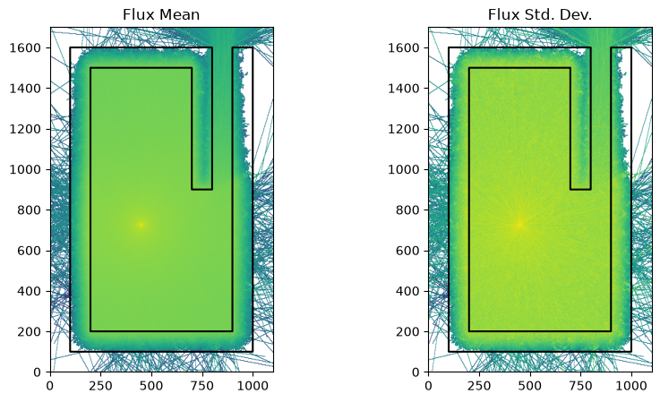
You might have to fine tune the particle numbers to get the two simulations taking exactly the same amount of time to make it a fair test.
However on this laptop both simulations took 30 seconds and it is clear from the two images that the weight window simulation was more efficient at getting particles through the shielding.
Weight windows can be fine tuned for a specific problem to improve their performance.
openmc.lib allows fine control over the weight window creation and that is covered in the next notebooks.