Survival Biasing Simulation#
This example simulates a shield room / bunker with a corridor entrance and a neutron source in the center of the room.
Variance reduction is used to accelerate the simulation.
The variance reduction method used for this simulation (survival_biasing) is not as effective as other variance reduction methods available in OpenMC but is the first task in the variance reduction section as it is the simplest to implement.
Openmc documentation on survival-biasing https://docs.openmc.org/en/stable/methods/neutron_physics.html#survival-biasing
First import OpenMC and configure the nuclear data path
import openmc
from matplotlib import pyplot as plt
from matplotlib.colors import LogNorm  # used for plotting log scale graphs
from pathlib import Path
# Setting the cross section path to the correct location in the docker image.
# If you are running this outside the docker image you will have to change this path to your local cross section path.
openmc.config['cross_sections'] = Path.home() / 'nuclear_data' / 'cross_sections.xml'
We create a couple of materials for the simulation
mat_air = openmc.Material(name="Air")
mat_air.add_element("N", 0.784431)
mat_air.add_element("O", 0.210748)
mat_air.add_element("Ar", 0.0046)
mat_air.set_density("g/cc", 0.001205)

mat_concrete = openmc.Material()
mat_concrete.add_element("H",0.168759)
mat_concrete.add_element("C",0.001416)
mat_concrete.add_element("O",0.562524)
mat_concrete.add_element("Na",0.011838)
mat_concrete.add_element("Mg",0.0014)
mat_concrete.add_element("Al",0.021354)
mat_concrete.add_element("Si",0.204115)
mat_concrete.add_element("K",0.005656)
mat_concrete.add_element("Ca",0.018674)
mat_concrete.add_element("Fe",0.00426)
mat_concrete.set_density("g/cm3", 2.3)

materials = openmc.Materials([mat_air, mat_concrete])
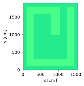
Now we define and plot the geometry. This geometry is defined by parameters for every width and height. The parameters input into the geometry in a stacked manner so they can easily be adjusted to change the geometry without creating overlapping cells.
width_a = 100
width_b = 200
width_c = 500
width_d = 250
width_e = 200
width_f = 200
width_g = 100

depth_a = 100
depth_b = 200
depth_c = 700
depth_d = 600
depth_e = 200
depth_f = 100

height_j = 100
height_k = 500
height_l = 100

xplane_0 = openmc.XPlane(x0=0, boundary_type="vacuum")
xplane_1 = openmc.XPlane(x0=xplane_0.x0 + width_a)
xplane_2 = openmc.XPlane(x0=xplane_1.x0 + width_b)
xplane_3 = openmc.XPlane(x0=xplane_2.x0 + width_c)
xplane_4 = openmc.XPlane(x0=xplane_3.x0 + width_d)
xplane_5 = openmc.XPlane(x0=xplane_4.x0 + width_e)
xplane_6 = openmc.XPlane(x0=xplane_5.x0 + width_f)
xplane_7 = openmc.XPlane(x0=xplane_6.x0 + width_g, boundary_type="vacuum")

yplane_0 = openmc.YPlane(y0=0, boundary_type="vacuum")
yplane_1 = openmc.YPlane(y0=yplane_0.y0 + depth_a)
yplane_2 = openmc.YPlane(y0=yplane_1.y0 + depth_b)
yplane_3 = openmc.YPlane(y0=yplane_2.y0 + depth_c)
yplane_4 = openmc.YPlane(y0=yplane_3.y0 + depth_d)
yplane_5 = openmc.YPlane(y0=yplane_4.y0 + depth_e)
yplane_6 = openmc.YPlane(y0=yplane_5.y0 + depth_f, boundary_type="vacuum")

zplane_1 = openmc.ZPlane(z0=0, boundary_type="vacuum")
zplane_2 = openmc.ZPlane(z0=zplane_1.z0 + height_j)
zplane_3 = openmc.ZPlane(z0=zplane_2.z0 + height_k)
zplane_4 = openmc.ZPlane(z0=zplane_3.z0 + height_l, boundary_type="vacuum")

outside_left_region = +xplane_0 & -xplane_1 & +yplane_1 & -yplane_5 & +zplane_1 & -zplane_4
wall_left_region = +xplane_1 & -xplane_2 & +yplane_2 & -yplane_4 & +zplane_2 & -zplane_3
wall_right_region = +xplane_5 & -xplane_6 & +yplane_2 & -yplane_5 & +zplane_2 & -zplane_3
wall_top_region = +xplane_1 & -xplane_4 & +yplane_4 & -yplane_5 & +zplane_2 & -zplane_3
outside_top_region = +xplane_0 & -xplane_7 & +yplane_5 & -yplane_6 & +zplane_1 & -zplane_4
wall_bottom_region = +xplane_1 & -xplane_6 & +yplane_1 & -yplane_2 & +zplane_2 & -zplane_3
outside_bottom_region = +xplane_0 & -xplane_7 & +yplane_0 & -yplane_1 & +zplane_1 & -zplane_4
wall_middle_region = +xplane_3 & -xplane_4 & +yplane_3 & -yplane_4 & +zplane_2 & -zplane_3
outside_right_region = +xplane_6 & -xplane_7 & +yplane_1 & -yplane_5 & +zplane_1 & -zplane_4

room_region = +xplane_2 & -xplane_3 & +yplane_2 & -yplane_4 & +zplane_2 & -zplane_3
gap_region = +xplane_3 & -xplane_4 & +yplane_2 & -yplane_3 & +zplane_2 & -zplane_3
corridor_region = +xplane_4 & -xplane_5 & +yplane_2 & -yplane_5 & +zplane_2 & -zplane_3

roof_region = +xplane_1 & -xplane_6 & +yplane_1 & -yplane_5 & +zplane_1 & -zplane_2
floor_region = +xplane_1 & -xplane_6 & +yplane_1 & -yplane_5 & +zplane_3 & -zplane_4

outside_left_cell = openmc.Cell(region=outside_left_region, fill=mat_air)
outside_right_cell = openmc.Cell(region=outside_right_region, fill=mat_air)
outside_top_cell = openmc.Cell(region=outside_top_region, fill=mat_air)
outside_bottom_cell = openmc.Cell(region=outside_bottom_region, fill=mat_air)
wall_left_cell = openmc.Cell(region=wall_left_region, fill=mat_concrete)
wall_right_cell = openmc.Cell(region=wall_right_region, fill=mat_concrete)
wall_top_cell = openmc.Cell(region=wall_top_region, fill=mat_concrete)
wall_bottom_cell = openmc.Cell(region=wall_bottom_region, fill=mat_concrete)
wall_middle_cell = openmc.Cell(region=wall_middle_region, fill=mat_concrete)
room_cell = openmc.Cell(region=room_region, fill=mat_air)
gap_cell = openmc.Cell(region=gap_region, fill=mat_air)
corridor_cell = openmc.Cell(region=corridor_region, fill=mat_air)

roof_cell = openmc.Cell(region=roof_region, fill=mat_concrete)
floor_cell = openmc.Cell(region=floor_region, fill=mat_concrete)

geometry = openmc.Geometry(
    [
        outside_bottom_cell,
        outside_top_cell,
        outside_left_cell,
        outside_right_cell,
        wall_left_cell,
        wall_right_cell,
        wall_top_cell,
        wall_bottom_cell,
        wall_middle_cell,
        room_cell,
        gap_cell,
        corridor_cell,
        roof_cell,
        floor_cell,
    ]
)
Now we plot the geometry and color by materials.
plot = geometry.plot(basis='xy', color_by='material')
plot.figure.savefig('geometry_top_down_view.png', bbox_inches="tight")
Next we create a point source, this also uses the same geometry parameters to place in the center of the room regardless of the values of the parameters.
# location of the point source
source_x = width_a + width_b + width_c * 0.5
source_y = depth_a + depth_b + depth_c * 0.75
source_z = height_j + height_k * 0.5
space = openmc.stats.Point((source_x, source_y, source_z))

angle = openmc.stats.Isotropic()

# all (100%) of source particles are 2.5MeV energy
energy = openmc.stats.Discrete([2.5e6], [1.0])

source = openmc.IndependentSource(space=space, angle=angle, energy=energy)
source.particle = "neutron"
Create a mesh that encompasses the entire geometry and scores neutron flux
mesh = openmc.RegularMesh().from_domain(geometry)
mesh.dimension = (100, 100, 1)

mesh_filter = openmc.MeshFilter(mesh)
particle_filter = openmc.ParticleFilter('neutron')

flux_tally = openmc.Tally(name="flux tally")
flux_tally.filters = [mesh_filter, particle_filter]
flux_tally.scores = ["flux"]

tallies = openmc.Tallies([flux_tally])
Creates the simulation settings
settings = openmc.Settings()

settings.run_mode = "fixed source"
settings.source = source
settings.particles = 2000
settings.batches = 5
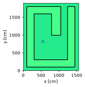
Creates the model and plot it to check the location of the source is correct
model = openmc.Model(geometry, materials, settings, tallies)

model.plot(n_samples=1, outline=True, color_by='material')
<Axes: xlabel='x [cm]', ylabel='y [cm]'>
We are going to run this model twice. Once with survival_biasing and once without. This next code bock makes a function so that we can easily run the simulation twice with these two different settings.
def run_and_plot(model: openmc.Model, image_filename: str) -> openmc.StatePoint:

    sp_filename = model.run()

    with openmc.StatePoint(sp_filename) as sp:
        flux_tally = sp.get_tally(name="flux tally")

    mesh_extent = mesh.bounding_box.extent['xy']

    # create a plot of the mean flux values
    flux_mean = flux_tally.get_reshaped_data(value='mean', expand_dims=True).squeeze()

    fig, (ax1, ax2) = plt.subplots(ncols=2, figsize=(10, 5))
    ax1.imshow(
        flux_mean.T,
        origin="lower",
        extent=mesh_extent,
        norm=LogNorm(),
    )

    ax1 = model.plot(
        outline='only',
        extent=model.bounding_box.extent['xz'],
        axes=ax1,  # Use the same axis as ax1\n",
        pixels=10_000_000,  #avoids rounded corners on outline
        color_by='material',
    )
    ax1.set_title("Flux Mean")

    # create a plot of the flux relative error
    flux_std_dev = flux_tally.get_reshaped_data(value='std_dev', expand_dims=True).squeeze()
    ax2.imshow(
        flux_std_dev.T,
        origin="lower",
        extent=mesh_extent,
        norm=LogNorm(),
    )

    ax2 = model.plot(
        outline='only',
        extent=model.bounding_box.extent['xz'],
        axes=ax2,  # Use the same axis as ax2\n",
        pixels=10_000_000,  #avoids rounded corners on outline
        color_by='material',
    )
    ax2.set_title("Flux Std. Dev.")

    plt.savefig(image_filename)
    return sp
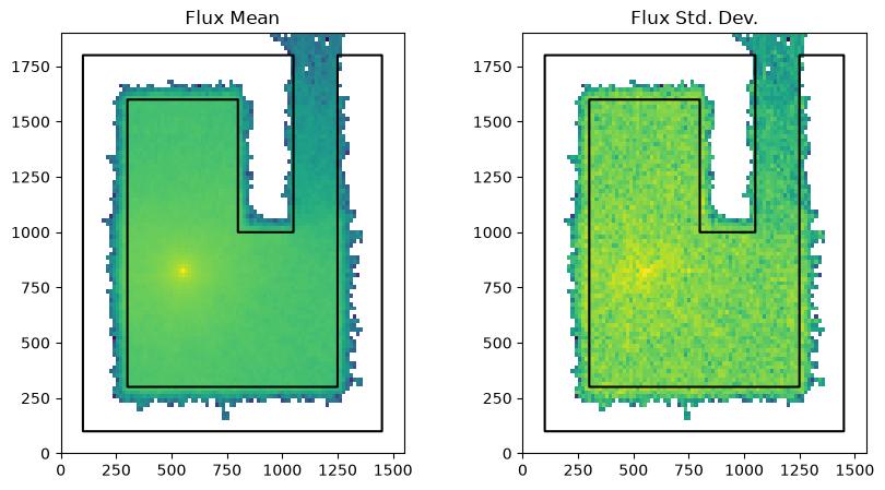
Now we run the model without survival_biasing and save the mesh tally image
run_and_plot(model, "no_survival_biasing.png")
                                %%%%%%%%%%%%%%%
                           %%%%%%%%%%%%%%%%%%%%%%%%
                        %%%%%%%%%%%%%%%%%%%%%%%%%%%%%%
                      %%%%%%%%%%%%%%%%%%%%%%%%%%%%%%%%%%
                    %%%%%%%%%%%%%%%%%%%%%%%%%%%%%%%%%%%%%%
                   %%%%%%%%%%%%%%%%%%%%%%%%%%%%%%%%%%%%%%%%
                                    %%%%%%%%%%%%%%%%%%%%%%%%
                                     %%%%%%%%%%%%%%%%%%%%%%%%
                 ###############      %%%%%%%%%%%%%%%%%%%%%%%%
                ##################     %%%%%%%%%%%%%%%%%%%%%%%
                ###################     %%%%%%%%%%%%%%%%%%%%%%%
                ####################     %%%%%%%%%%%%%%%%%%%%%%
                #####################     %%%%%%%%%%%%%%%%%%%%%
                ######################     %%%%%%%%%%%%%%%%%%%%
                #######################     %%%%%%%%%%%%%%%%%%
                 #######################     %%%%%%%%%%%%%%%%%
                 ######################     %%%%%%%%%%%%%%%%%
                  ####################     %%%%%%%%%%%%%%%%%
                    #################     %%%%%%%%%%%%%%%%%
                     ###############     %%%%%%%%%%%%%%%%
                       ############     %%%%%%%%%%%%%%%
                          ########     %%%%%%%%%%%%%%
                                      %%%%%%%%%%%

                 | The OpenMC Monte Carlo Code
       Copyright | 2011-2026 MIT, UChicago Argonne LLC, and contributors
         License | https://docs.openmc.org/en/latest/license.html
         Version | 0.15.3-dev485
     Commit Hash | 6704e4786a743611baac5d693943f67f7479ee47
       Date/Time | 2026-06-17 21:41:05
  OpenMP Threads | 4

 Reading model XML file 'model.xml' ...
 Reading cross sections XML file...
 Reading N14 from /home/runner/nuclear_data/neutron/N14.h5
 Reading N15 from /home/runner/nuclear_data/neutron/N15.h5
 Reading O16 from /home/runner/nuclear_data/neutron/O16.h5
 Reading O17 from /home/runner/nuclear_data/neutron/O17.h5
 Reading O18 from /home/runner/nuclear_data/neutron/O18.h5
 Reading Ar36 from /home/runner/nuclear_data/neutron/Ar36.h5
 WARNING: Negative value(s) found on probability table for nuclide Ar36 at 294K
 Reading Ar38 from /home/runner/nuclear_data/neutron/Ar38.h5
 Reading Ar40 from /home/runner/nuclear_data/neutron/Ar40.h5
 Reading H1 from /home/runner/nuclear_data/neutron/H1.h5
 Reading H2 from /home/runner/nuclear_data/neutron/H2.h5
 Reading C12 from /home/runner/nuclear_data/neutron/C12.h5
 Reading C13 from /home/runner/nuclear_data/neutron/C13.h5
 Reading Na23 from /home/runner/nuclear_data/neutron/Na23.h5
 Reading Mg24 from /home/runner/nuclear_data/neutron/Mg24.h5
 Reading Mg25 from /home/runner/nuclear_data/neutron/Mg25.h5
 Reading Mg26 from /home/runner/nuclear_data/neutron/Mg26.h5
Reading Al27 from /home/runner/nuclear_data/neutron/Al27.h5
Reading Si28 from /home/runner/nuclear_data/neutron/Si28.h5
Reading Si29 from /home/runner/nuclear_data/neutron/Si29.h5
 Reading Si30 from /home/runner/nuclear_data/neutron/Si30.h5
 Reading K39 from /home/runner/nuclear_data/neutron/K39.h5
 Reading K40 from /home/runner/nuclear_data/neutron/K40.h5
 Reading K41 from /home/runner/nuclear_data/neutron/K41.h5
 Reading Ca40 from /home/runner/nuclear_data/neutron/Ca40.h5
 Reading Ca42 from /home/runner/nuclear_data/neutron/Ca42.h5
 Reading Ca43 from /home/runner/nuclear_data/neutron/Ca43.h5
 Reading Ca44 from /home/runner/nuclear_data/neutron/Ca44.h5
 Reading Ca46 from /home/runner/nuclear_data/neutron/Ca46.h5
 Reading Ca48 from /home/runner/nuclear_data/neutron/Ca48.h5
Reading Fe54 from /home/runner/nuclear_data/neutron/Fe54.h5
Reading Fe56 from /home/runner/nuclear_data/neutron/Fe56.h5
Reading Fe57 from /home/runner/nuclear_data/neutron/Fe57.h5
Reading Fe58 from /home/runner/nuclear_data/neutron/Fe58.h5
 Minimum neutron data temperature: 294.0 K
 Maximum neutron data temperature: 294.0 K
 Preparing distributed cell instances...
 Writing summary.h5 file...
 Maximum neutron transport energy: 20000000.0 eV for N15

 ===============>     FIXED SOURCE TRANSPORT SIMULATION     <===============

 Simulating batch 1
Simulating batch 2
 Simulating batch 3
 Simulating batch 4
 Simulating batch 5
 Creating state point statepoint.5.h5...
 =======================>     TIMING STATISTICS     <=======================

 Total time for initialization     = 3.9821e+00 seconds
   Reading cross sections          = 3.9578e+00 seconds
 Total time in simulation          = 9.9680e-01 seconds
   Time in transport only          = 9.8712e-01 seconds
   Time in active batches          = 9.9680e-01 seconds
   Time accumulating tallies       = 1.8709e-03 seconds
   Time writing statepoints        = 6.9537e-03 seconds
 Total time for finalization       = 9.4064e-03 seconds
 Total time elapsed                = 4.9933e+00 seconds
 Calculation Rate (active)         = 10032.1 particles/second

 ============================>     RESULTS     <============================

 Leakage Fraction            = 0.00360 +/- 0.00064
<openmc.statepoint.StatePoint at 0x7f19bd1a9460>
Now we run the model again with survival_biasing enabled. This needs to be set on the model settings. The values chosen can be fine tuned to the model but for this example we have chosen some values after a little exploration.
model.settings.survival_biasing = True
model.settings.cutoff = {
    "weight": 0.3,  # value needs to be between 0 and 1
    "weight_avg": 0.9,  # value needs to be between 0 and 1
}
run_and_plot(model, "yes_survival_biasing.png")
                                %%%%%%%%%%%%%%%
                           %%%%%%%%%%%%%%%%%%%%%%%%
                        %%%%%%%%%%%%%%%%%%%%%%%%%%%%%%
                      %%%%%%%%%%%%%%%%%%%%%%%%%%%%%%%%%%
                    %%%%%%%%%%%%%%%%%%%%%%%%%%%%%%%%%%%%%%
                   %%%%%%%%%%%%%%%%%%%%%%%%%%%%%%%%%%%%%%%%
                                    %%%%%%%%%%%%%%%%%%%%%%%%
                                     %%%%%%%%%%%%%%%%%%%%%%%%
                 ###############      %%%%%%%%%%%%%%%%%%%%%%%%
                ##################     %%%%%%%%%%%%%%%%%%%%%%%
                ###################     %%%%%%%%%%%%%%%%%%%%%%%
                ####################     %%%%%%%%%%%%%%%%%%%%%%
                #####################     %%%%%%%%%%%%%%%%%%%%%
                ######################     %%%%%%%%%%%%%%%%%%%%
                #######################     %%%%%%%%%%%%%%%%%%
                 #######################     %%%%%%%%%%%%%%%%%
                 ######################     %%%%%%%%%%%%%%%%%
                  ####################     %%%%%%%%%%%%%%%%%
                    #################     %%%%%%%%%%%%%%%%%
                     ###############     %%%%%%%%%%%%%%%%
                       ############     %%%%%%%%%%%%%%%
                          ########     %%%%%%%%%%%%%%
                                      %%%%%%%%%%%

                 | The OpenMC Monte Carlo Code
       Copyright | 2011-2026 MIT, UChicago Argonne LLC, and contributors
         License | https://docs.openmc.org/en/latest/license.html
         Version | 0.15.3-dev485
     Commit Hash | 6704e4786a743611baac5d693943f67f7479ee47
       Date/Time | 2026-06-17 21:41:14
  OpenMP Threads | 4

 Reading model XML file 'model.xml' ...
 Reading cross sections XML file...
 Reading N14 from /home/runner/nuclear_data/neutron/N14.h5
 Reading N15 from /home/runner/nuclear_data/neutron/N15.h5
 Reading O16 from /home/runner/nuclear_data/neutron/O16.h5
 Reading O17 from /home/runner/nuclear_data/neutron/O17.h5
 Reading O18 from /home/runner/nuclear_data/neutron/O18.h5
 Reading Ar36 from /home/runner/nuclear_data/neutron/Ar36.h5
 WARNING: Negative value(s) found on probability table for nuclide Ar36 at 294K
 Reading Ar38 from /home/runner/nuclear_data/neutron/Ar38.h5
 Reading Ar40 from /home/runner/nuclear_data/neutron/Ar40.h5
 Reading H1 from /home/runner/nuclear_data/neutron/H1.h5
 Reading H2 from /home/runner/nuclear_data/neutron/H2.h5
 Reading C12 from /home/runner/nuclear_data/neutron/C12.h5
 Reading C13 from /home/runner/nuclear_data/neutron/C13.h5
 Reading Na23 from /home/runner/nuclear_data/neutron/Na23.h5
 Reading Mg24 from /home/runner/nuclear_data/neutron/Mg24.h5
 Reading Mg25 from /home/runner/nuclear_data/neutron/Mg25.h5
 Reading Mg26 from /home/runner/nuclear_data/neutron/Mg26.h5
Reading Al27 from /home/runner/nuclear_data/neutron/Al27.h5
Reading Si28 from /home/runner/nuclear_data/neutron/Si28.h5
Reading Si29 from /home/runner/nuclear_data/neutron/Si29.h5
 Reading Si30 from /home/runner/nuclear_data/neutron/Si30.h5
 Reading K39 from /home/runner/nuclear_data/neutron/K39.h5
 Reading K40 from /home/runner/nuclear_data/neutron/K40.h5
 Reading K41 from /home/runner/nuclear_data/neutron/K41.h5
 Reading Ca40 from /home/runner/nuclear_data/neutron/Ca40.h5
 Reading Ca42 from /home/runner/nuclear_data/neutron/Ca42.h5
 Reading Ca43 from /home/runner/nuclear_data/neutron/Ca43.h5
 Reading Ca44 from /home/runner/nuclear_data/neutron/Ca44.h5
 Reading Ca46 from /home/runner/nuclear_data/neutron/Ca46.h5
 Reading Ca48 from /home/runner/nuclear_data/neutron/Ca48.h5
Reading Fe54 from /home/runner/nuclear_data/neutron/Fe54.h5
Reading Fe56 from /home/runner/nuclear_data/neutron/Fe56.h5
Reading Fe57 from /home/runner/nuclear_data/neutron/Fe57.h5
Reading Fe58 from /home/runner/nuclear_data/neutron/Fe58.h5
 Minimum neutron data temperature: 294.0 K
 Maximum neutron data temperature: 294.0 K
 Preparing distributed cell instances...
 Writing summary.h5 file...
 Maximum neutron transport energy: 20000000.0 eV for N15

 ===============>     FIXED SOURCE TRANSPORT SIMULATION     <===============

 Simulating batch 1
Simulating batch 2
Simulating batch 3
Simulating batch 4
Simulating batch 5
 Creating state point statepoint.5.h5...

 =======================>     TIMING STATISTICS     <=======================

 Total time for initialization     = 3.8759e+00 seconds
   Reading cross sections          = 3.8520e+00 seconds
 Total time in simulation          = 1.3927e+00 seconds
   Time in transport only          = 1.3855e+00 seconds
   Time in active batches          = 1.3927e+00 seconds
   Time accumulating tallies       = 7.4358e-05 seconds
   Time writing statepoints        = 6.4620e-03 seconds
 Total time for finalization       = 1.0094e-02 seconds
 Total time elapsed                = 5.2838e+00 seconds
 Calculation Rate (active)         = 7180.46 particles/second

 ============================>     RESULTS     <============================

 Leakage Fraction            = 0.00486 +/- 0.00066
<openmc.statepoint.StatePoint at 0x7f19bcdeb740>
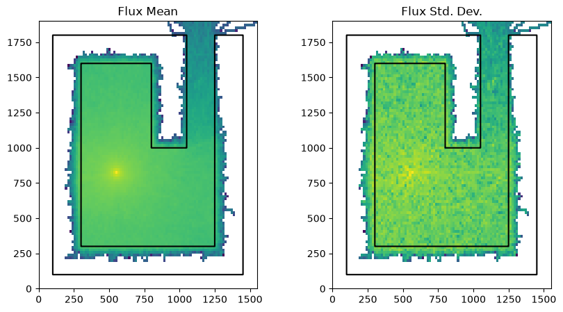
Comparing the two simulations we notice that the survival_biasing simulation resulted in slightly improved flux tally and a slightly improved standard deviation.
This model is used again in the next example that makes use of weight windows and yields more impressive acceleration.