Build-up Factors

Why they're needed

The point-kernel method computes uncollided flux: particles that travel straight from source to detector without any interaction. In reality, scattered particles also reach the detector, adding to the dose. The build-up factor \(B\) corrects for this:

\[\Phi_{\text{total}} = \Phi_{\text{uncollided}} \cdot B\]

For shielding design, ignoring build-up is non-conservative; it underestimates the dose.

Properties of B

• \(B \geq 1\) always (scattered particles add dose, never subtract)
• \(B\) increases with shield thickness (thicker shields scatter more)
• \(B\) depends on material (hydrogenous materials have larger \(B\))
• \(B\) depends on energy and particle type
• \(B\) depends on layer ordering in multi-layer shields

Why not use tabulated data?

Traditional approaches (ANSI/ANS-6.4.3, Hila et al.) provide pre-computed build-up factors, but they have fundamental limitations:

• Energy binning: Tabulated values are computed at discrete energies and interpolated. Cross sections have resonance structure that this misses, especially for neutrons where removal cross sections are isotope-specific.
• Material mixing: Tables exist per element (photons) or per isotope (neutrons), but real shields are compounds. Combining elemental \(B\) values needs a mixing rule (Harima, Bremer-Roussin, Broder), all of which are approximate because buildup depends on the correlated scatter history through the material. A photon that Compton-scatters on hydrogen and then photoelectric-absorbs on iron is not represented in either pure-H or pure-Fe tables. The error is small when constituent Z values are similar or one element dominates the cross section, and largest when the compound mixes low-Z (Compton) and high-Z (photoelectric) elements in comparable amounts (e.g. heavy concrete with steel rebar, or tungsten-loaded polymers), or when the photon energy sits near a K-edge.
• Geometry specificity: Tabulated \(B\) values are for infinite homogeneous media. Real multi-layer shields have \(B\) that depends on layer ordering; two different layer combinations with the same total optical thickness can have different \(B\) values.

Our approach: Monte Carlo computed B

Instead, this tool computes \(B\) directly from Monte Carlo simulation for the user's exact geometry:

\[B = \frac{\text{MC dose (total, all scattering)}}{\text{PK dose (uncollided only)}}\]

OpenMC runs full particle transport with pointwise cross sections (no energy binning), tracking every scatter and energy loss. The ratio MC/PK gives the exact build-up factor for that specific geometry, material combination, and source energy.

Advantages:

• Pointwise energy treatment: OpenMC uses continuous-energy cross sections, capturing all resonance structure
• Exact geometry: \(B\) is computed for the user's specific layer stack, not a generic infinite medium
• Statistical uncertainty: Each Monte Carlo result comes with a standard deviation, which propagates through to the final dose estimate
• Works for any material: No need for pre-computed tables per element; any user-defined composition works

Analytical-form fit and extrapolation

Running Monte Carlo for every thickness is expensive. The workflow is:

1. Run Monte Carlo on a few thin shields (e.g. 4-6 thicknesses) - these are cheap to simulate
2. Fit a closed-form expression to the \(B\) values vs thickness, weighted by the Monte Carlo statistical uncertainty
3. Predict \(B\) at any thickness by evaluating the fitted form

BuildupFit uses two forms depending on the input dimensionality:

• 1D (single material): Shin-Ishii / Taylor double-exponential \(B(\mu t) = A \cdot e^{-\alpha_1 \mu t} + (1 - A) \cdot e^{-\alpha_2 \mu t}\). Three free parameters with \(B(0) = 1\) baked in. Validated empirically to capture growth, decay, peak-and-decay (light multipliers like beryllium), and dip-and-recover all with one functional form. The literature precedent is Shin & Ishii (1990s) for neutrons in concrete and iron; the same form was Taylor's original photon expression.
• Multi-D (multi-layer geometries): thin-plate-spline RBF with degree-1 polynomial augmentation. No hyperparameters; works on scattered points.

Each Monte Carlo data point has a statistical uncertainty \(\sigma_B\) that the fit uses for weighted least squares: tight points pull the fit harder than noisy ones.

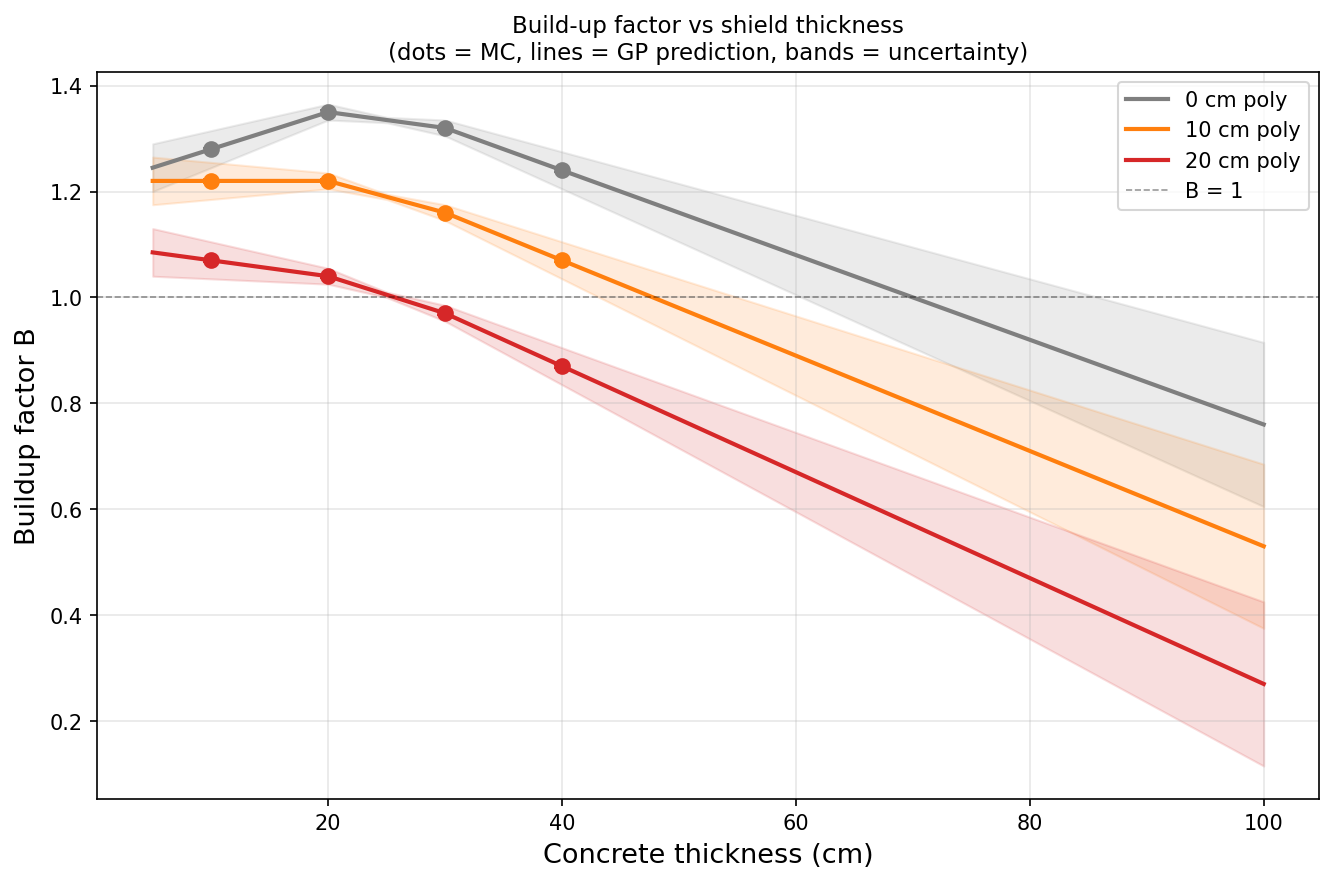
Build-up factor vs concrete thickness for different water thicknesses. Dots are Monte Carlo simulations with error bars. Lines are the fitted forms.

Flux vs dose build-up

Build-up factors for flux and dose are different:

• \(B_{\text{flux}}\): Corrects particle count (all scattered particles regardless of energy)
• \(B_{\text{dose}}\): Corrects dose (scattered particles weighted by their energy-dependent dose coefficient)

Since scattered particles have lower energies and dose coefficients change with energy, \(B_{\text{flux}} \neq B_{\text{dose}}\) in general. For shielding design, use dose build-up.

Effect of build-up on flux estimates

Without build-up correction, the point-kernel method underestimates the flux, especially for thick shields where scattered particles dominate:

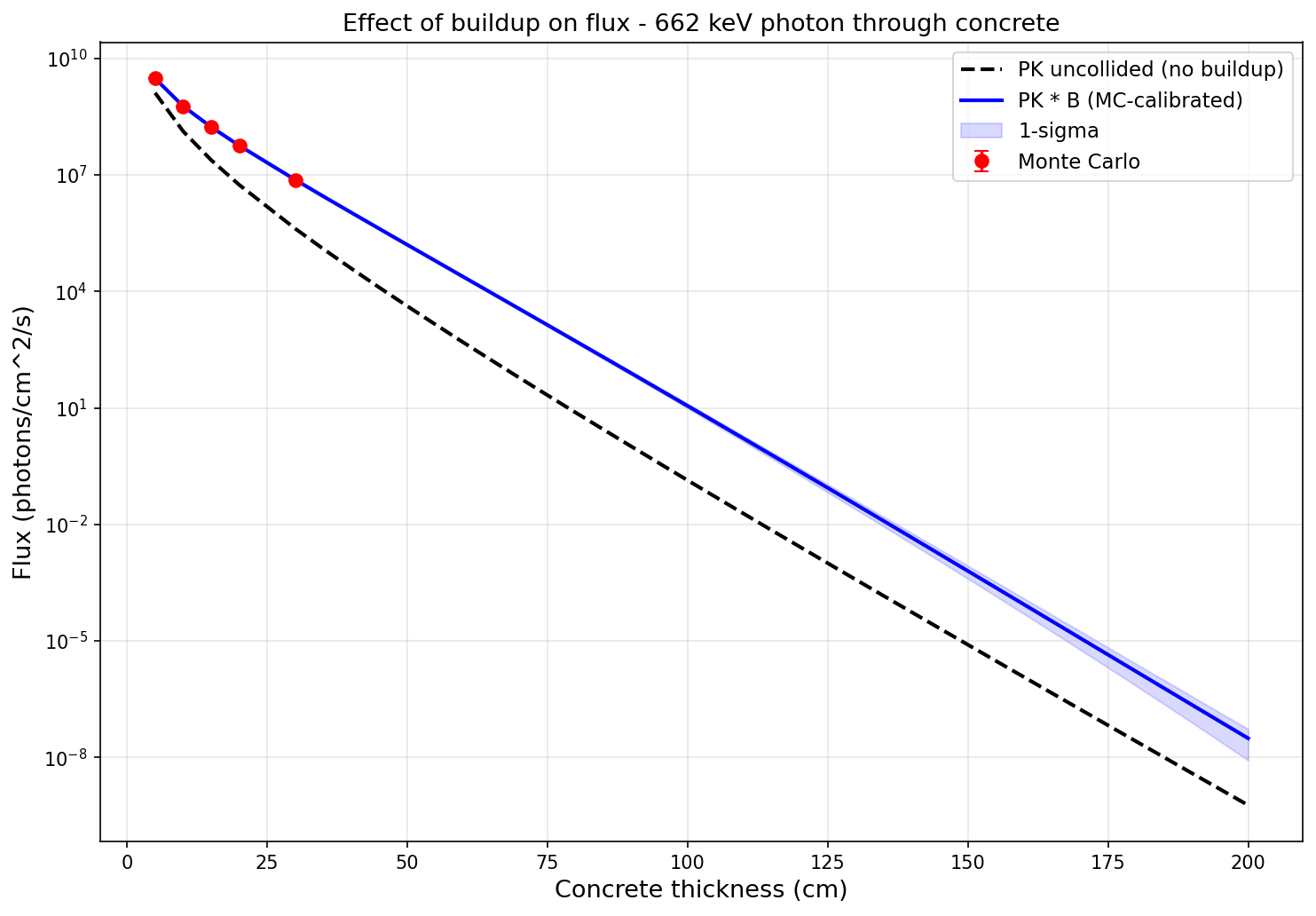
Flux vs shield thickness for a 662 keV photon source through concrete. The PK uncollided estimate (dashed) increasingly underestimates the true flux as thickness grows; \(B_{\text{flux}}\) counts every scattered particle regardless of energy.

Effect of build-up on dose estimates

The same effect applies to dose, though smaller than for flux because \(B_{\text{dose}}\) weights scattered particles by their (lower) dose coefficient while \(B_{\text{flux}}\) counts them all:

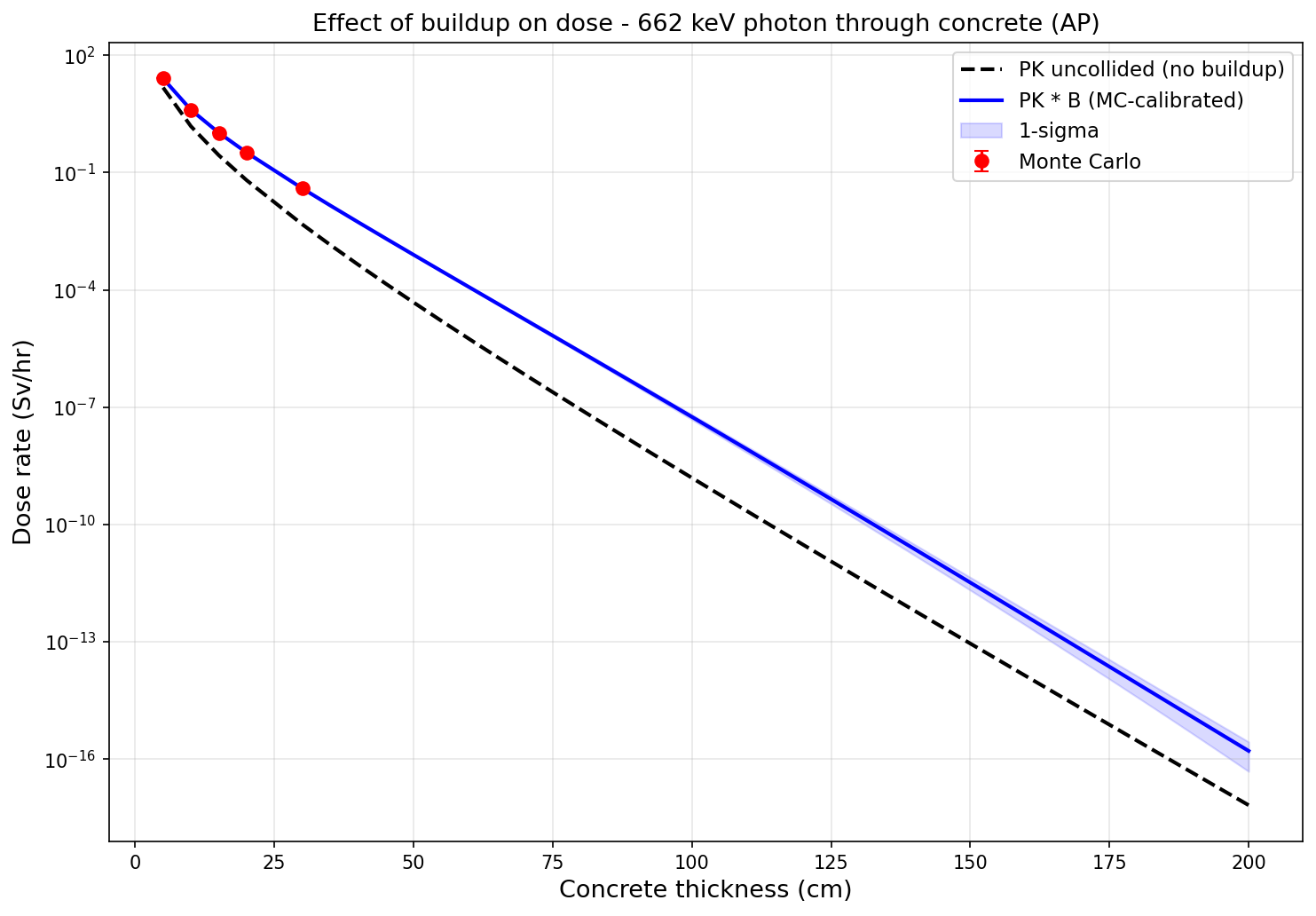
Dose rate vs shield thickness for the same source and shield. The dashed line (PK uncollided) underestimates compared to the solid line (PK with Monte Carlo build-up correction). Monte Carlo simulation points confirm the corrected estimate. \(B_{\text{dose}}\) is typically 0.5-0.7x smaller than \(B_{\text{flux}}\) at the same thickness.